AMIETE – ET (NEW SCHEME) – Code: AE61
Subject: CONTROL ENGINEERING
 Time: 3 Hours
Max. Marks: 100
Time: 3 Hours
Max. Marks: 100
NOTE: There are 9 Questions in all.
· Question 1 is compulsory and
carries 20 marks. Answer to Q. 1 must be written in the space provided for it
in the answer book supplied and nowhere else.
· Out of the remaining EIGHT
Questions, answer any FIVE Questions. Each question carries 16 marks.
· Any required data not
explicitly given, may be suitably assumed and stated.
Q.1 Choose the correct or the best alternative in the following: (2![]() 10)
10)
a.
A disc
of inertia J initially at rest acted upon by a torque T(t) as shown in Fig.1, is described by
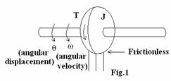
(A) ![]() (B)
(B) ![]()
(C) ![]() (D)
(D) ![]()
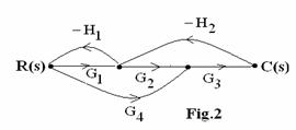
b.
The number of feedback loops present
in
the signal flow graph of Fig.2, is
(A) 1 (B) 2
(C) 3 (D) 4
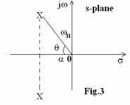
c. For the
pole-zero plot of Fig.3, the
damping ratio ![]() is given by
is given by
(A) ![]() (B)
(B)
![]()
(C) ![]() (D)
(D) ![]()
d. If the root-locus of a system
with
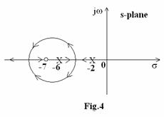
![]() is a circle as shown
in
is a circle as shown
in
Fig.4,
then
(A) K is negative
(B) number of asymptotes is 0
(C) plot will not cut the imaginary
axis
(D) all of the above.
e. A system whose characteristic equation is ![]() will be stable by
Routh-Hurwitz criterion, if
will be stable by
Routh-Hurwitz criterion, if
(A) K>0 (B) K>2
(C) ![]() (D) K>3
(D) K>3
f. The
undamped natural frequency ![]() of a system with
of a system with ![]() is
is
(A)
![]() (B)
(B) ![]()
(C) ![]() (D)
(D) ![]()
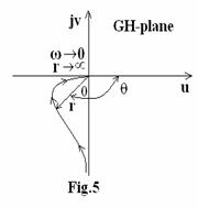
g. The transfer
function G(s) corresponding
to the polar
plot of Fig.5, is of the form
(A) ![]() (B)
(B) ![]()
(C) ![]() (D)
(D) ![]()
h. The instantaneous rms value of
voltage![]() proportional to the rotor speed
proportional to the rotor speed ![]() developed on a
tachometer with sensitivity
developed on a
tachometer with sensitivity ![]() is given by
is given by
(A) ![]() (B)
(B)
![]()
(C) ![]() (D)
(D) ![]()
i. A linear
system described by the differential equation![]() ,
with
,
with ![]() as the state variables
has the state model
as the state variables
has the state model
(A)
 (B)
(B) 
(C)  (D)
(D) 
j. Consider a
nonlinear system described by![]() ,
,![]() , with
, with ![]() and a possible
Liapunov function
and a possible
Liapunov function ![]() . The system is
. The system is
(A) unstable (B) having unstable limit cycles
(C) locally stable or
stable-in-the-small (D) asymptotically stable
Answer any FIVE Questions out
of EIGHT Questions.
Each question carries 16
marks.
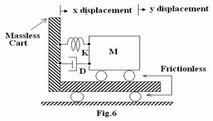
Q.2 a. For the mechanical system of Fig.6, draw the
free-body diagram and write the differential equation of the system. Draw the
electrical analogue using force-voltage analogy. (8)
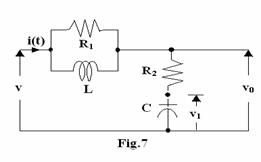
b. For the electrical network as shown in Fig.7,
write the
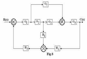
Q.3 a. Using block-diagram reduction technique,
obtain the overall transfer function for the system as shown in Fig.8. (8)
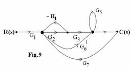
b. Applying Mason’s gain formula obtain the overall transfer
function for the signal-flow graph as shown in Fig.9. (8)
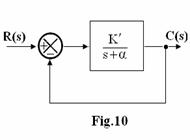
Q.4 a. Consider
the feedback system shown in Fig.10, with time-constant
![]() and
and ![]() . (i) Sketch the
closed-loop system response c(t) for an impulse input
. (i) Sketch the
closed-loop system response c(t) for an impulse input ![]() . (ii) Show that the
effect of feedback is to increase the bandwidth. (4+4)
. (ii) Show that the
effect of feedback is to increase the bandwidth. (4+4)
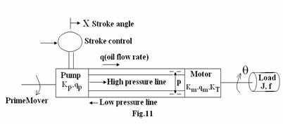
b. Derive the
transfer function ![]() of the hydraulic
pump-motor system described by Fig.11, where
of the hydraulic
pump-motor system described by Fig.11, where ![]() are constants,
p=pressure drop across the motor,
are constants,
p=pressure drop across the motor, ![]() =coefficient of compressibility,
=coefficient of compressibility, ![]() = angle through which the motor turns,
= angle through which the motor turns, ![]() =leakage oil flow rate. (8)
=leakage oil flow rate. (8)
Q.5 a. A second-order unity feedback control system
has an open-loop transfer function ![]() . By what factor
should the amplifier gain A be multiplied so that
. By what factor
should the amplifier gain A be multiplied so that
(i) The damping ratio ![]() is
increased from a value of 0.2 to 0.6?
is
increased from a value of 0.2 to 0.6?
(ii) The
overshoot of the unit step response is reduced from 80% to 20%? (4+4)
b.
A signal ![]() actuates a control system described by
actuates a control system described by  , where K is a constant and
 ![]() . Apply Routh-Hurwitz
criterion to the characteristic equation 1+E(s) = 0 and find the value of K to
keep the system stable. Assume zero
initial conditions. (8)
. Apply Routh-Hurwitz
criterion to the characteristic equation 1+E(s) = 0 and find the value of K to
keep the system stable. Assume zero
initial conditions. (8)
Q.6 a. Consider
the unity feedback control system with![]() . Sketch the
root-locus on a graph sheet, and determine the damping factor. Find the
corresponding value of K. (8)
. Sketch the
root-locus on a graph sheet, and determine the damping factor. Find the
corresponding value of K. (8)
b. Consider
the root ![]() for nominal gain
for nominal gain ![]() for the system
for the system![]() . Compute the root
sensitivity to K, z and p. (8)
. Compute the root
sensitivity to K, z and p. (8)
Q.7
a. Construct the Nyquist plot and determine the stability of the system![]() . (10)
. (10)
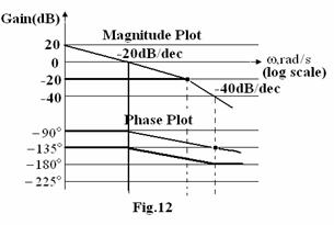
b. Define
gain margin and phase margin. From the
Bode plot diagram drawn in Fig.12, determine the gain margin and phase margin.
State whether the system is stable. (6)
Q.8 a. A
unity feedback type-2 system with ![]() has its closed-loop
poles always lying on the
has its closed-loop
poles always lying on the ![]() -axis on its root-locus.
It is desired to compensate the system to satisfy that settling time
-axis on its root-locus.
It is desired to compensate the system to satisfy that settling time ![]() and damping factor
and damping factor![]() . Indicate on the
s-plane the locations for the compensator pole and zero and obtain the
open-loop transfer function
. Indicate on the
s-plane the locations for the compensator pole and zero and obtain the
open-loop transfer function![]() . (8)
. (8)
b. For each
compensator-lead, lag, lag-lead, write (i)
typical electrical network, (ii) s-plane representation and (iii)
transfer function. Explain the need for compensation networks in control
systems. (6+2)
Q.9 a. Determine the state controllability and
observability of the linear system, described by the equation ![]() where
where ![]() (8)
(8)
b. The state
equation of a linear time-invariant system is represented by: ![]() Write the characteristic
equation and obtain the state transition matrix
Write the characteristic
equation and obtain the state transition matrix![]() . (8)
. (8)