AMIETE – ET (OLD SCHEME)
 Code: AE11 Subject:
CONTROL ENGINEERING
Code: AE11 Subject:
CONTROL ENGINEERING
Time: 3 Hours Max. Marks: 100
NOTE: There are 9 Questions in all.
· Question 1 is compulsory and
carries 20 marks. Answer to Q.1 must be written in the space provided for it in
the answer book supplied and nowhere else.
· Out of the remaining EIGHT
Questions, answer any FIVE Questions. Each question carries 16 marks.
· Any required data not
explicitly given, may be suitably assumed and stated.
Q.1 Choose
the correct or the best alternative in the following: (2![]() 10)
10)
a. For the system ![]() letting
letting ![]() as
as ![]() ,
, ![]()
(A) ![]() a small angle (B)
a small angle (B) ![]() a small angle
a small angle
(C) ![]() a small angle (D)
a small angle (D) ![]() a small angle
a small angle
b. For the inertia-damper rotational system with a rigid shaft shown in Fig. 1 the torque equation is:
(A)
0.2s![]() (B)
(B) ![]()
(C) ![]() (D)
(D)
![]()
c.
The output c(t) for an impulse
input r(t)= ![]() for the system of Fig.
2 is:
for the system of Fig.
2 is:
(A) ![]() (B)
(B) ![]()
(C) ![]() (D)
(D) ![]()
d. The time constant of the second order-system ![]() is:
is:
(A) 0.2s (B) 12s
(C) 60s (D) 10s
e.
The origin for the frequency response
plot is (0 dB gain, –180![]() phase) in:
phase) in:
(A)
Root-locus (B) Nichols chart
(C) Nyquist plot (D)
None of these
f. The type of the system and the velocity
error constant ![]() for the system with
for the system with ![]() are given by:
are given by:
(A) 1 and ![]() (B) 1 and
(B) 1 and ![]()
(C) 1 and ![]() (D)
1 and
(D)
1 and ![]()
g. The point of intersection of the asymptotes
(centroid) for the root-locus of the system![]() , is:
, is:
(A) 0 (B)
2
(C) 3 (D) 5
h. Application of Routh-Hurwitz criterion to the
system of Fig. 3 shows that it will be unstable for:
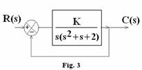
(A) ![]() (B)
(B)
![]()
(C) ![]() (D)
(D)
![]()
i. The basic circuit of Fig. 4 represents a:
(A) lag compensator
(B) lead compensator
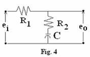
(C) lag-lead compensator
(D) lead-lag compensator
j. While using digital implementation of analog
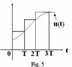
compensators, the integral approximation
procedure shown in Fig. 5 is called:
(A) forward rectangular rule
(B)
forward difference approximator
(C) trapezoidal rule
(D) backward rectangular rule
Answer any FIVE Questions out of EIGHT
Questions.
Each question carries 16
marks.
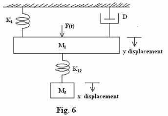
Q.2 a. Consider an external force F(t) applied
to mass M1 as in Fig. 6. Write the free- body diagram and the
differential equations. Draw the electrical equivalent network using
force-current analogy. (8)
b. With a neat
diagram, explain the function of an ac tacho-generator and obtain its transfer
function. (8)
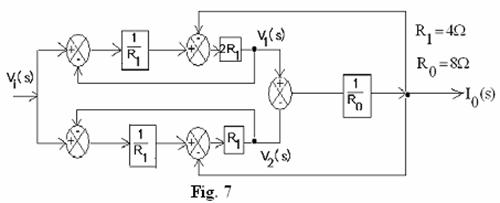
Q.3 a.
Using block-diagram reduction technique, find the closed-loop transfer function
of Fig 7. (8)
b. Obtain the overall transfer function of the
system whose signal-flow graph is shown in Fig. 8, using Mason’s gain formula. (8)
Q.4 a. Consider the feedback control system of Fig. 9
with a disturbance input W(s). Show that feedback reduces the effect of
disturbance on the controlled output. Obtain the sensitivity function S(j![]() ) of the system and the disturbance transfer function
) of the system and the disturbance transfer function![]() .
How is disturbance rejection accomplished? (8)
.
How is disturbance rejection accomplished? (8)
b. Determine the damping ratio ![]() and the values of ‘a’
and ‘b’ if the first overshoot is 16% and time-constant is 0.1 sec for the system
forward path transfer function G(S)= 10/S2 and feed back H(S)=
(as+b). (8)
and the values of ‘a’
and ‘b’ if the first overshoot is 16% and time-constant is 0.1 sec for the system
forward path transfer function G(S)= 10/S2 and feed back H(S)=
(as+b). (8)
Q.5 a. Use Routh stability criterion to check the stability of systems
with characteristic equation: (i)![]() , and show (ii)
, and show (ii) ![]() has all roots with
real parts more negative than –1. (8)
has all roots with
real parts more negative than –1. (8)
b. For the unity feedback system: ![]() state the type of the
system and identify its poles and zeros. Determine the steady state errors for
a unit step input, a unit ramp input and an acceleration input,
state the type of the
system and identify its poles and zeros. Determine the steady state errors for
a unit step input, a unit ramp input and an acceleration input, ![]() . If this system is required to follow a parabolic input
signal, will it perform satisfactorily? (8)
. If this system is required to follow a parabolic input
signal, will it perform satisfactorily? (8)
Q.6 a. Draw a typical passive electrical network and the pole-zero plot,
and write the transfer function for each type of compensator: lead, lag and
lag-lead. Explain the need for compensation networks in control systems. (8)
b. Sketch
the root-locus for a unity feedback system having forward path transfer
function as![]() and find the value
of K when the root-locus cuts the
and find the value
of K when the root-locus cuts the ![]() -axis. (8)
-axis. (8)
Q.7 a. For a standard second order system  , show that the phase-margin is given by
  . Calculate
![]() . What will be the approximation for
. What will be the approximation for ![]() for low values of
damping ratio
for low values of
damping ratio ![]() ? (8)
? (8)
b. Sketch the
Nyquist plot and determine the stability of the system ![]() (8)
(8)
Q.8 a. The transfer function of a lead compensator
is given by ![]() Find the magnitude of
Find the magnitude of ![]() at the frequency
at the frequency ![]() of maximum phase lead
of maximum phase lead ![]() and express
and express ![]() in terms of
in terms of ![]() . If
. If ![]() (8)
(8)
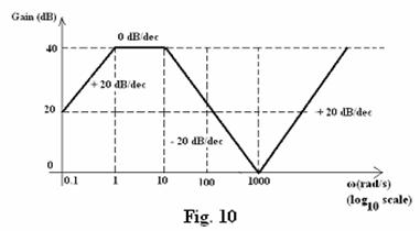
b. Obtain
the open-loop transfer function of the system whose Bode magnitude plot is
shown in Fig. 10. (8)
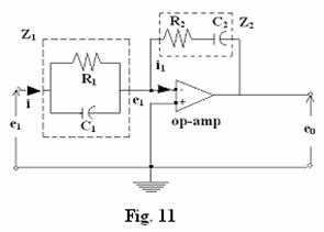
Q.9 a. Consider
the circuit of Fig. 11 with an ideal op-amp. Derive the transfer function in
terms of: (i) ![]() (ii) circuit elements.
Show that the circuit process the input signal by “proportional + integral +
derivative” action. (8)
(ii) circuit elements.
Show that the circuit process the input signal by “proportional + integral +
derivative” action. (8)
b. What is a
robust control system? List the model uncertainty factors that should be
considered to make the system design robust. (8)